Gemma 4 Architecture Explained: Per-Layer Embeddings, Shared KV Cache, and Dual RoPE

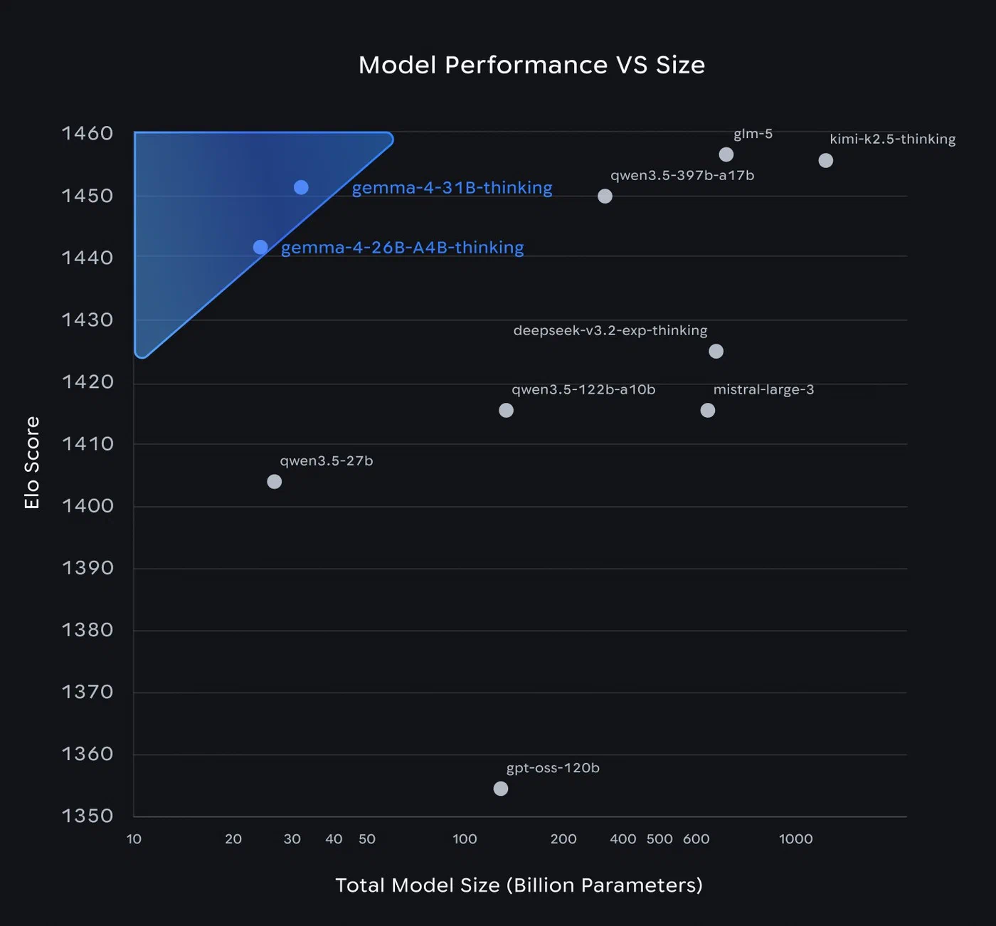
Gemma 4 , released on April 2, 2026, ships four model variants under the Apache 2.0 license. The 31B dense model ranks third on the Arena AI text leaderboard with a score of 1452. The 26B MoE model scores 1441 while activating only 3.8B of its 26B total parameters per forward pass. These numbers raise the obvious question: what architectural decisions make this possible? Three specific design choices - Per-Layer Embeddings (PLE), Shared KV Cache, and Dual RoPE - break from the standard transformer recipe in ways that have real consequences for inference cost, memory footprint, and fine-tuning strategy. The rest of this post covers those mechanisms, the Mixture-of-Experts layer, and the multimodal encoders.
What the Standard Transformer Does (and Where It Falls Short)
A standard transformer decoder works like this: a single embedding table maps token IDs to vectors. Those vectors pass through N identical decoder layers, each containing self-attention (Q, K, V projections, attention computation, output projection) and a feed-forward network (FFN). At the end, an output head produces next-token probabilities.
Two properties of this design matter for understanding Gemma 4’s changes:
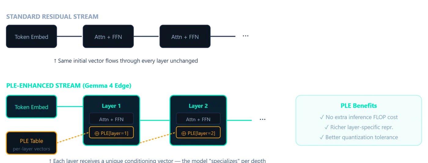
- One embedding, used once. The token embedding is consumed at the input layer. Every subsequent layer transforms the same residual stream, and the original token identity signal degrades as it passes through dozens of layers.
- Independent KV cache per layer. Each layer computes and stores its own key and value tensors during autoregressive generation. Memory scales as
layers x sequence_length x hidden_dim. At 256K context with 30+ layers, this becomes the dominant memory bottleneck - easily exceeding 24 GB on a single GPU.
Standard Rotary Position Embeddings (RoPE) apply the same frequency scheme uniformly across all layers. This works fine when every layer sees the full context, but Gemma 4 alternates between local sliding-window and global full-context layers, and a single RoPE configuration is suboptimal for both.
Per-Layer Embeddings: A Second Embedding Table for Every Layer
Per-Layer Embeddings (PLE) first appeared in Gemma 3n and returns in Gemma 4’s edge models (E2B and E4B). The idea is straightforward: instead of one embedding table consumed at input, PLE adds a parallel, lower-dimensional conditioning pathway that feeds a small dedicated vector into every decoder layer.
For each token, PLE produces a per-layer vector by combining two signals:
- A token-identity component from a second embedding lookup table
- A context-aware component from a learned projection of the main embeddings
Each decoder layer receives its corresponding PLE vector and uses it to modulate the hidden states via a lightweight residual addition after attention and feed-forward computation. This gives each layer its own channel to receive token-specific information when it becomes relevant, rather than forcing the initial embedding to front-load everything the model might ever need.
The parameter cost is real. The E2B model has 2.3B effective parameters but 5.1B total parameters - the PLE table accounts for much of that difference. The E4B model shows a similar ratio: 4.5B effective, 8B total with embeddings. But the inference cost is minimal, since PLE is a lookup plus an addition per layer, not a matrix multiply.
There is a practical wrinkle with multimodal data, though. For images, audio, and video, PLE is computed before soft tokens are merged into the embedding sequence. Since PLE relies on discrete token IDs that are lost once multimodal features replace the placeholders, multimodal positions receive the pad token ID, which effectively gives them neutral per-layer signals.
The 26B and 31B models do not use PLE. It is specifically an efficiency technique for smaller models where the parameter budget is tight and per-layer specialization helps compensate for reduced model capacity.
Shared KV Cache: Reusing Key-Value Tensors Across Layers
The KV cache is the primary memory bottleneck for long-context inference. In a standard transformer, layer L computes its own K_L and V_L tensors from its input, and these are cached for autoregressive generation. Every layer maintains independent key-value storage.
Gemma 4’s Shared KV Cache changes this for the 26B and 31B models. The last num_kv_shared_layers layers do not compute their own key and value projections. Instead, they reuse the K and V tensors from the last non-shared layer of the same attention type (sliding-window or full-context).
The key details:
- Shared layers still compute their own Q (query) tensors. Only K and V are reused.
- The sharing respects the attention type boundary: sliding-window layers share with other sliding-window layers, and global layers share with other global layers.
- Memory savings scale with the number of shared layers. If 10 of 30 layers share KV tensors, KV cache memory drops by roughly 33%.
Why does this work without destroying quality? Research on deep transformers has shown that K/V representations in later layers converge toward similar patterns. The last several layers of a deep network often compute near-identical attention distributions. Sharing their KV tensors formalizes this observation and eliminates redundant computation.
This is a different optimization from Grouped Query Attention (GQA), which reduces KV cache by sharing across attention heads within a single layer. Gemma 4 uses both: GQA reduces per-layer cache size, while Shared KV Cache reduces the number of layers that need independent cache storage. The two are orthogonal.
The practical result: you can run 256K context on a consumer GPU with 24 GB VRAM. At Q4_K_M quantization, the 26B MoE model needs about 15 GB, leaving headroom for the KV cache even at long context lengths.
Dual RoPE: Two Position Encoding Strategies in One Model
Gemma 4 alternates between two types of attention layers:
- Local sliding-window layers that attend to a fixed window (512 tokens for E2B/E4B, 1024 tokens for 26B/31B)
- Global full-context layers that attend to the entire sequence (up to 128K or 256K tokens)
Applying standard RoPE to both layer types creates a compromise. Local layers do not need long-range position signals - they benefit from sharp, precise discrimination between nearby positions. Global layers need position encodings that maintain quality across hundreds of thousands of tokens, where standard RoPE frequencies cause very distant tokens to receive near-zero attention weights (the “attention sink” problem).
Gemma 4 solves this with Dual RoPE:
- Local layers use standard RoPE with a base frequency tuned for short-range attention
- Global layers use proportional RoPE (p-RoPE), which scales the base frequency proportionally to the maximum context length
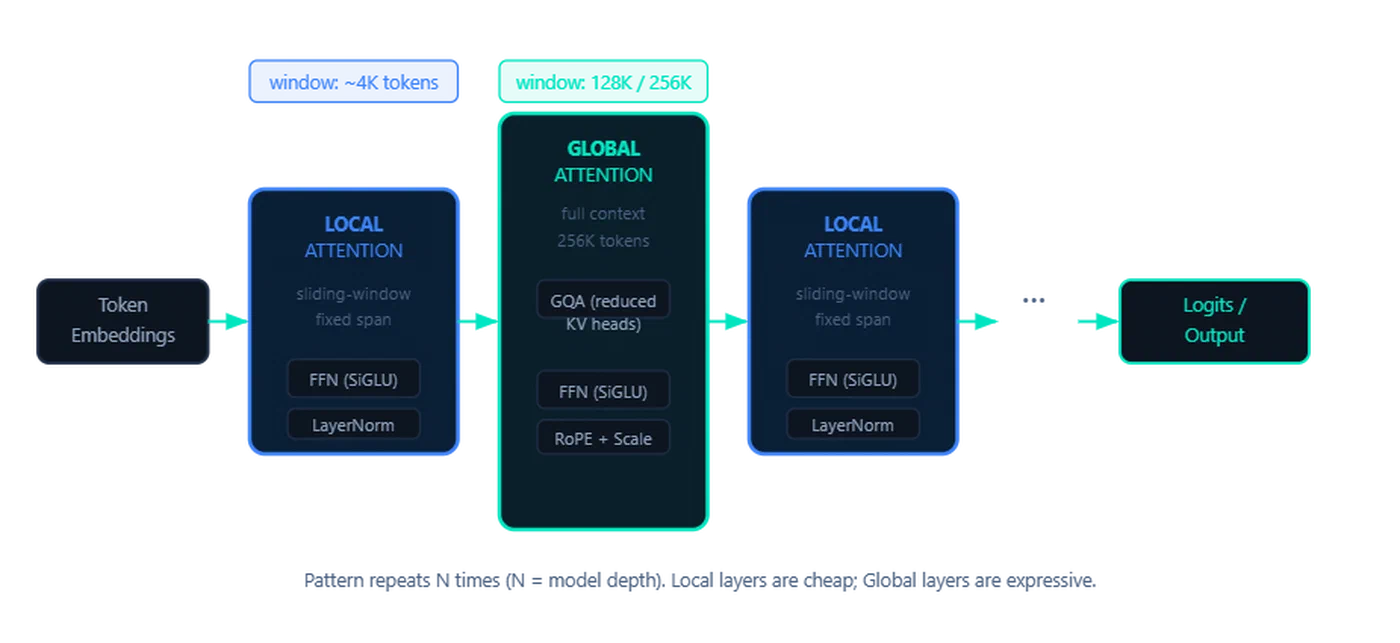
p-RoPE prevents attention quality degradation at extreme distances by adjusting how quickly the rotation angles change with position. Using p-RoPE everywhere would blur nearby position discrimination in local layers, so the dual approach gives each layer type the position encoding scheme it actually needs.
For comparison, Llama 4
uses standard RoPE with rope_scaling for extended context, and Qwen 2.5
uses YaRN. Both are single-strategy approaches that make a global tradeoff. Gemma 4’s dual approach avoids that compromise by matching the encoding to each layer’s attention range.
The MoE Layer: 128 Experts, 8 Active, 1 Shared
The 26B A4B variant replaces the standard FFN in each decoder layer with a Mixture-of-Experts (MoE) feed-forward network. Each MoE layer contains:
- 128 specialist experts: small FFN modules, each trained on different data patterns
- 1 shared expert: always active, handles common patterns like punctuation and basic syntax
- A learned router: a gating network that selects the top-8 experts per token based on the token’s representation
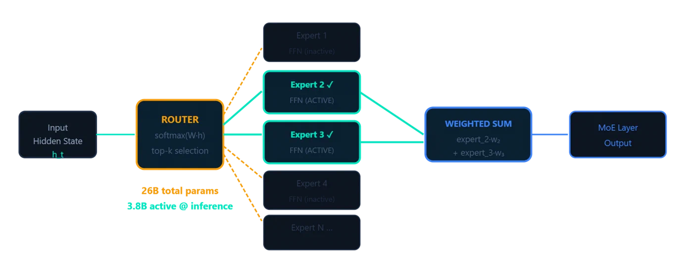
The math on active parameters: 8 of 128 specialist experts fire per token, plus the shared expert, plus all attention layers. That totals roughly 3.8B active parameters per forward pass out of 26B total. All 128 experts must be loaded into memory, but only a fraction performs computation for any given token.
| Metric | 26B MoE (A4B) | 31B Dense |
|---|---|---|
| Total Parameters | 26B | 31B |
| Active Parameters | 3.8B | 31B |
| Context Window | 256K | 256K |
| LMArena Score | 1441 | 1452 |
| AIME 2026 | ~85% | 89.2% |
| MMLU Pro | ~83% | 85.2% |
Different experts learn different domains. Some activate primarily for code, others for natural language, others for mathematical reasoning. A load-balancing loss during training prevents “expert collapse” - the failure mode where the router sends everything to a few experts while most sit unused.
The inference speed advantage is significant: the 26B MoE model generates tokens at roughly the speed of a 4B dense model, since only 3.8B parameters are active per forward pass. But memory bandwidth becomes the real bottleneck on consumer hardware. All expert weights must be resident in VRAM even though most are idle for any given token. The RTX 4090 at 960 GB/s bandwidth handles this well; Apple Silicon at ~400 GB/s on M4 Max is more constrained.
For comparison, Llama 4 Maverick uses 128 experts with 1 shared expert but activates 17B of 400B parameters - much larger scale, same principle.
Vision and Audio Encoders
Gemma 4 processes images, video, and audio through dedicated encoders that feed into the main transformer.
Vision encoder:
- ~150M parameters for E2B/E4B, ~550M for 26B/31B
- Learned 2D positional embeddings with multidimensional RoPE, preserving spatial relationships
- Configurable token budget: 70, 140, 280, 560, or 1120 tokens per image, allowing a quality-speed tradeoff
- Original aspect ratio preservation - images are not force-resized to squares
- Video processing (26B/31B only): frames sampled at 1fps, each processed by the vision encoder, up to 60 seconds
Audio encoder (E2B/E4B only):
- ~300M parameters, USM-style conformer architecture
- Trained on speech data only (no music or environmental sounds)
- Same base architecture as the one in Gemma 3n
The modality split across variants is a bit awkward: the 26B/31B models handle video but not audio, while E2B/E4B handle audio but not video. No single Gemma 4 model covers text, image, video, and audio in one pass.
Vision and audio tokens are interleaved with text tokens in the input sequence, allowing cross-attention between modalities within the main transformer. This is standard practice for modern multimodal models, but the configurable image token budget is a practical differentiator - you can trade off image understanding quality against inference speed by choosing how many tokens to spend per image.
What This Means for Inference and Fine-Tuning
Each architectural choice creates practical consequences for deployment.
The PLE secondary embedding table is trainable on its own. You can fine-tune per-layer token representations independently from the main weights, which opens up a lightweight specialization path for the edge models without full-weight fine-tuning.
On context length, Gemma 4’s reduced cache memory means you can push longer contexts on less VRAM than comparable models like Qwen 3.5 or Llama 4 Scout. The savings stack with quantization - Q4_K_M on a 24 GB GPU leaves meaningful room for KV cache at 256K context. But extending beyond 256K tokens would require adjusting both RoPE variants separately. This is not as simple as changing a single rope_scaling parameter, which makes community-driven context extensions more complex than for single-RoPE models.
Fine-tuning the 26B MoE raises questions that dense models do not. Do you tune the router, the shared expert, all 128 experts, or just the active ones? Unsloth recommends targeting attention projections plus the shared expert FFN for the best quality-cost tradeoff. This avoids the combinatorial problem of tuning 128 specialist experts while still adapting the model’s core behavior.
Batched MoE inference is trickier than batched dense inference. Different tokens in a batch may activate different experts, so the working set of active experts varies across the batch. This matters for serving infrastructure - vLLM and similar frameworks need to account for expert activation patterns.
Prompt caching also behaves differently with Gemma 4’s alternating attention pattern. Local sliding-window layers do not benefit from full prompt caching since they only attend to a fixed window of recent tokens. Only global layers cache the full prompt, so the effective cache hit rate depends on the ratio of global to local layers.
Gemma 4 Model Comparison
| Feature | E2B | E4B | 26B A4B (MoE) | 31B Dense |
|---|---|---|---|---|
| Total Params | 5.1B | 8B | 26B | 31B |
| Effective/Active Params | 2.3B | 4.5B | 3.8B | 31B |
| Architecture | Dense + PLE | Dense + PLE | MoE | Dense |
| Context Window | 128K | 128K | 256K | 256K |
| Sliding Window | 512 tokens | 512 tokens | 1024 tokens | 1024 tokens |
| Per-Layer Embeddings | Yes | Yes | No | No |
| Shared KV Cache | No | No | Yes | Yes |
| Vision Encoder | ~150M params | ~150M params | ~550M params | ~550M params |
| Audio Support | Yes | Yes | No | No |
| Video Support | No | No | Yes | Yes |
| Target Hardware | Phones | Edge/IoT | Consumer GPU | Data Center |
Google did not publish ablation studies isolating the contribution of each architectural component. The published benchmark numbers reflect the full architecture combined with the training recipe, so we cannot say exactly how many points PLE or Shared KV Cache individually contribute. Community evaluations are ongoing, and independent ablation results may surface as researchers dig into the open weights.
What we can say is that the overall design philosophy is pragmatic. Google explicitly dropped more exotic features like Altup in favor of components that are “highly compatible across libraries and devices” - good news for anyone wanting to run these models with existing tooling on commodity hardware.