Gemma 4 Architecture Explained: Per-Layer Embeddings, Shared KV Cache, and Dual RoPE

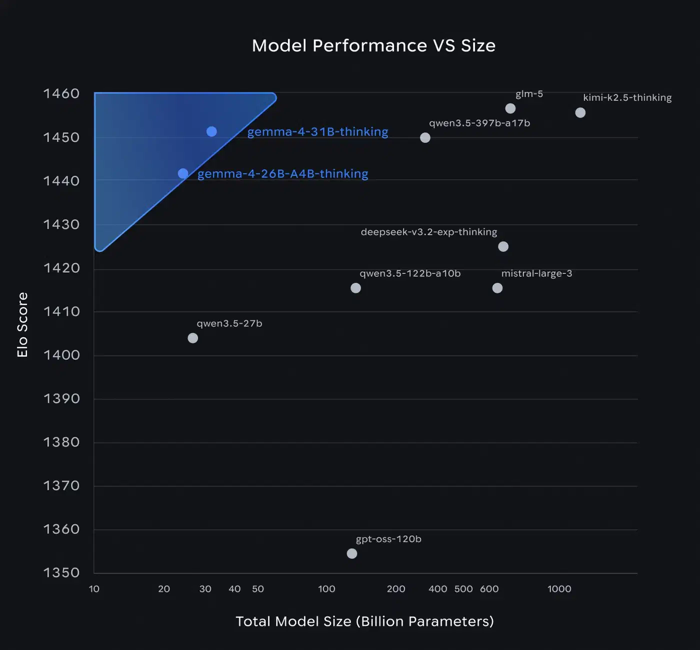
Gemma 4 shipped on April 2, 2026 with four model variants under the Apache 2.0 license. The 31B dense model ranks third on the Arena AI text leaderboard with a score of 1452. The 26B MoE model scores 1441 while firing only 3.8B of its 26B total parameters per forward pass. So what design choices make this possible? Three of them break from the standard transformer recipe: Per-Layer Embeddings (PLE), Shared KV Cache, and Dual RoPE. Each one shifts the math for inference cost, memory use, and fine-tuning. The rest of this post covers those three, plus the Mixture-of-Experts layer and the multimodal encoders.
What the Standard Transformer Does (and Where It Falls Short)
A standard transformer decoder works like this. A single embedding table maps token IDs to vectors. Those vectors pass through N identical decoder layers. Each layer has self-attention (Q, K, V projections, the attention math, and an output projection) plus a feed-forward network (FFN). At the end, an output head gives next-token probabilities.
Two properties of this design set up Gemma 4’s changes:
- One embedding, used once. The token embedding is read at the input layer. Every later layer reshapes the same residual stream, and the original token identity signal fades as it passes through dozens of layers.
- Independent KV cache per layer. Each layer builds and stores its own key and value tensors during generation. Memory scales as
layers x sequence_length x hidden_dim. At 256K context with 30+ layers, this is the main memory drain. It can easily go past 24 GB on a single GPU.
Standard Rotary Position Embeddings (RoPE) apply the same frequency scheme to every layer. That works fine when every layer sees the full context. However, Gemma 4 alternates between local sliding-window layers and global full-context layers. A single RoPE setup is a poor fit for both.
Per-Layer Embeddings: A Second Embedding Table for Every Layer
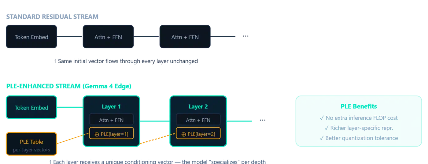
Per-Layer Embeddings (PLE) first showed up in Gemma 3n and returns in Gemma 4’s edge models (E2B and E4B). The idea is simple. Instead of one embedding table read at the input, PLE adds a side channel. It feeds a small dedicated vector into every decoder layer.
For each token, PLE produces a per-layer vector by combining two signals:
- A token-identity component from a second embedding lookup table
- A context-aware component from a learned projection of the main embeddings
Each decoder layer gets its own PLE vector and uses it to tweak the hidden states. The tweak is a light residual add after attention and the feed-forward step. So each layer has its own line for token-specific signal, fed in when it helps. The input embedding no longer has to pre-pack every fact the model might need later.
The parameter cost is real. The E2B model has 2.3B active parameters but 5.1B total parameters. The PLE table soaks up most of that gap. The E4B model has the same kind of ratio: 4.5B active, 8B total with embeddings. The inference cost stays tiny though, since PLE is one lookup plus one add per layer, not a matrix multiply.
There is a wrinkle for multimodal data, though. For images, audio, and video, PLE runs before soft tokens are merged into the embedding sequence. PLE needs discrete token IDs, but those IDs are gone once multimodal features take the place of the slots. So multimodal positions get the pad token ID, which gives them flat per-layer signals.
The 26B and 31B models skip PLE. It is a trick for smaller models, where the parameter budget is tight and per-layer specialization helps make up for lower model capacity.
Shared KV Cache: Reusing Key-Value Tensors Across Layers
The KV cache is the main memory drag for long-context inference. In a standard transformer, layer L builds its own K_L and V_L tensors from its input. Those tensors are cached for generation. Every layer keeps its own key-value store.
Gemma 4’s Shared KV Cache changes this for the 26B and 31B models. The last num_kv_shared_layers layers skip their own key and value projections. They reuse the K and V tensors from the last non-shared layer of the same attention type (sliding-window or full-context).
The key details:
- Shared layers still compute their own Q (query) tensors. Only K and V are reused.
- The sharing respects the attention type boundary: sliding-window layers share with other sliding-window layers, and global layers share with other global layers.
- Memory savings scale with the number of shared layers. If 10 of 30 layers share KV tensors, KV cache memory drops by roughly 33%.
Why does this not hurt quality? Work on deep transformers has shown that K/V values in later layers tend to drift toward the same patterns. The last few layers of a deep network often build near-identical attention maps. Sharing their KV tensors bakes that fact into the model and skips the duplicate work.
This is a different fix from Grouped Query Attention (GQA), which cuts KV cache by sharing across attention heads inside one layer. Gemma 4 uses both. GQA cuts per-layer cache size, while Shared KV Cache cuts the number of layers that need their own cache. The two stack.
The practical result: you can run 256K context on a consumer GPU with 24 GB VRAM . At Q4_K_M quantization , the 26B MoE model needs about 15 GB. That leaves headroom for the KV cache, even at long context lengths.
Dual RoPE: Two Position Encoding Strategies in One Model
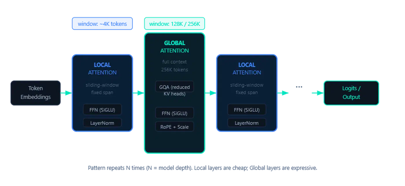
Gemma 4 alternates between two types of attention layers:
- Local sliding-window layers that attend to a fixed window (512 tokens for E2B/E4B, 1024 tokens for 26B/31B)
- Global full-context layers that attend to the entire sequence (up to 128K or 256K tokens)
Applying standard RoPE to both layer types is a compromise. Local layers do not need long-range position signals. They want sharp, crisp splits between nearby positions. Global layers need position codes that hold up across hundreds of thousands of tokens. With standard RoPE, very distant tokens get near-zero attention weights (the “attention sink” problem).
Gemma 4 solves this with Dual RoPE:
- Local layers use standard RoPE with a base frequency tuned for short-range attention
- Global layers use proportional RoPE (p-RoPE), which scales the base frequency proportionally to the maximum context length
p-RoPE keeps attention sharp at extreme distances by tuning how fast the rotation angles change with position. Using p-RoPE everywhere would blur nearby position splits in local layers. So the dual approach gives each layer type the encoding scheme it needs.
For comparison, Llama 4
uses standard RoPE with rope_scaling for long context, and Qwen 2.5
uses YaRN. Both are single-strategy moves that make one global tradeoff. Gemma 4’s dual approach skips that tradeoff and matches the encoding to each layer’s attention range.
The MoE Layer: 128 Experts, 8 Active, 1 Shared
The 26B A4B variant swaps the standard FFN in each decoder layer for a Mixture-of-Experts (MoE) feed-forward network. Each MoE layer has:
- 128 specialist experts: small FFN modules, each trained on different data patterns
- 1 shared expert: always active, handles common patterns like punctuation and basic syntax
- A learned router: a gating network that selects the top-8 experts per token based on the token’s representation
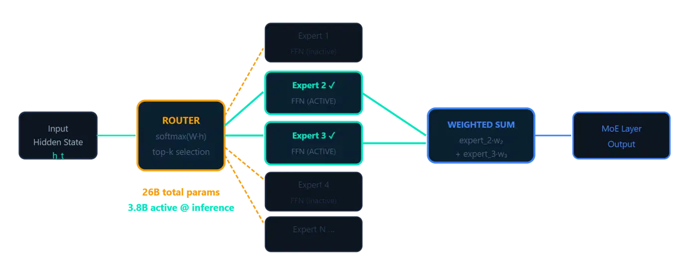
The math on active parameters: 8 of 128 specialist experts fire per token, plus the shared expert, plus all attention layers. That adds up to about 3.8B active parameters per forward pass out of 26B total. All 128 experts have to be loaded in memory, but only a few run the math for any given token.
| Metric | 26B MoE (A4B) | 31B Dense |
|---|---|---|
| Total Parameters | 26B | 31B |
| Active Parameters | 3.8B | 31B |
| Context Window | 256K | 256K |
| LMArena Score | 1441 | 1452 |
| AIME 2026 | ~85% | 89.2% |
| MMLU Pro | ~83% | 85.2% |
Different experts learn different domains. Some fire mostly for code, others for natural language, others for math. A load-balancing loss during training blocks “expert collapse.” That is the failure mode where the router sends everything to a few experts while most sit idle.
The speed gain is big. The 26B MoE model produces tokens at about the speed of a 4B dense model, since only 3.8B parameters are active per forward pass. However, memory bandwidth turns into the real bottleneck on consumer hardware. All expert weights have to live in VRAM even though most are idle for any given token. The RTX 4090 at 960 GB/s handles this well. Apple Silicon at about 400 GB/s on M4 Max is tighter.
For comparison, Llama 4 Maverick uses 128 experts with 1 shared expert but fires 17B of 400B parameters. Much bigger scale, same idea.
Vision and Audio Encoders
Gemma 4 handles images, video, and audio through dedicated encoders that feed into the main transformer.
Vision encoder:
- About 150M parameters for E2B/E4B, about 550M for 26B/31B
- Learned 2D position embeddings with multi-axis RoPE, which keeps spatial layout intact
- Tunable token budget: 70, 140, 280, 560, or 1120 tokens per image, for a quality-speed tradeoff
- Keeps the original aspect ratio. Images are not forced into squares.
- Video (26B/31B only): frames sampled at 1fps, each run through the vision encoder, up to 60 seconds
Audio encoder (E2B/E4B only):
- About 300M parameters, USM-style conformer design
- Trained on speech data only (no music or background sounds)
- Same base design as the one in Gemma 3n
The modality split across variants is a bit odd. The 26B/31B models handle video but not audio, while E2B/E4B handle audio but not video. No single Gemma 4 model covers text, image, video, and audio in one pass.
Vision and audio tokens are mixed in with text tokens in the input sequence. That lets cross-attention work across modalities inside the main transformer. This is standard for modern multimodal models. The tunable image token budget is the real differentiator. You can trade off image quality for inference speed by picking how many tokens to spend per image.
What This Means for Inference and Fine-Tuning
Each design choice has knock-on effects for how you deploy the model.
The PLE side embedding table is trainable on its own. You can fine-tune per-layer token vectors apart from the main weights. That opens a lightweight tuning path for the edge models without touching the full set of weights.
On context length, Gemma 4’s smaller cache means you can push longer contexts on less VRAM than peers like Qwen 3.5 or Llama 4 Scout
. The savings stack with quantization. Q4_K_M on a 24 GB GPU leaves real room for KV cache at 256K context. Going past 256K tokens would mean tuning both RoPE variants on their own. That is harder than flipping a single rope_scaling value, which makes community context extensions trickier than for single-RoPE models.
Fine-tuning the 26B MoE raises questions that dense models do not. Do you tune the router, the shared expert, all 128 experts, or just the active ones? Unsloth says target the attention projections plus the shared expert FFN for the best quality-cost ratio. That sidesteps the combo problem of tuning 128 specialist experts and still shifts the model’s core behavior.
Batched MoE inference is trickier than batched dense inference. Different tokens in a batch can fire different experts, so the set of active experts shifts across the batch. That has real effects on serving setup. vLLM and other frameworks need to plan for these activation patterns.
Prompt caching also works differently with Gemma 4’s alternating attention pattern. Local sliding-window layers do not get much from full prompt caching, since they only look at a fixed window of recent tokens. Only global layers cache the full prompt. So the real cache hit rate depends on the ratio of global to local layers.
Gemma 4 Model Comparison
| Feature | E2B | E4B | 26B A4B (MoE) | 31B Dense |
|---|---|---|---|---|
| Total Params | 5.1B | 8B | 26B | 31B |
| Effective/Active Params | 2.3B | 4.5B | 3.8B | 31B |
| Architecture | Dense + PLE | Dense + PLE | MoE | Dense |
| Context Window | 128K | 128K | 256K | 256K |
| Sliding Window | 512 tokens | 512 tokens | 1024 tokens | 1024 tokens |
| Per-Layer Embeddings | Yes | Yes | No | No |
| Shared KV Cache | No | No | Yes | Yes |
| Vision Encoder | ~150M params | ~150M params | ~550M params | ~550M params |
| Audio Support | Yes | Yes | No | No |
| Video Support | No | No | Yes | Yes |
| Target Hardware | Phones | Edge/IoT | Consumer GPU | Data Center |
Google did not publish ablation studies that isolate each piece of the design. The published benchmark numbers come from the full setup plus the training recipe. So we cannot say how many points PLE or Shared KV Cache add on their own. Community evals are ongoing, and outside ablation results may show up as researchers dig into the open weights.
What we can say is that the design choices are pragmatic. Google dropped more exotic features like Altup in favor of parts that are “highly compatible across libraries and devices.” That is good news for anyone running these models on stock tooling and commodity hardware.