AI-Powered Log Analysis: Find Anomalies in Server Logs with Local LLMs

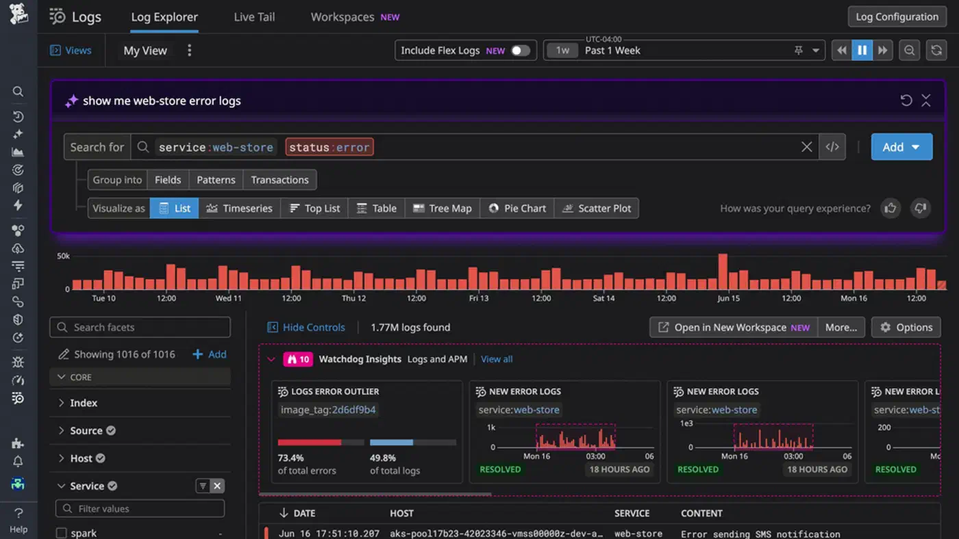
You can use a local LLM like Llama 3.3 70B or Qwen 2.5 32B running through Ollama to analyze structured server logs faster and more contextually than traditional grep/awk workflows. By piping parsed log data through a prompt that instructs the model to identify anomalous patterns, correlate error cascades, and generate root-cause hypotheses, you get incident summaries and actionable insights within seconds. This covers the gap between simple text search and expensive commercial observability platforms like Datadog or Splunk , all without sending sensitive log data off your network.

Why LLMs Beat Grep for Log Analysis

Pattern-based tools like grep, awk, and jq require you to already know the error string or pattern you are looking for. That works great when you know what broke. It falls apart when the problem is something you have never seen before or when the symptom is a subtle shift in behavior rather than an explicit error message.

LLMs can identify anomalies by understanding context. A 10x spike in 200 OK responses with 3-second latencies is completely invisible to grep - there is no error string to match. But a model prompted to find “unusual patterns” in structured log data will flag that immediately, because it understands that 3-second response times for endpoints that normally return in 50ms is abnormal even though the HTTP status code is technically fine.

LLMs also correlate events across services well. If you feed interleaved logs from nginx, a Python backend, and PostgreSQL into a single prompt, the model can identify that a database connection pool exhaustion at 14:32:05 caused the 502 errors that started two seconds later at 14:32:07. Doing that manually with grep means jumping between three different log files and mentally reconstructing the timeline. The LLM does it in one pass.

The practical sweet spot for LLM log analysis is post-incident investigation and ad-hoc exploration. This is not a replacement for real-time alerting. A 70B model takes 10-30 seconds to process 5,000 log lines, which is perfectly fine when you are doing a post-mortem but far too slow for a streaming pipeline that needs sub-second response times. Use Loki and Grafana Alloy for log aggregation and retention, Grafana for dashboards and alerting, and then point an LLM at a specific time window when something looks wrong. The LLM is the analyst, not the monitoring system.

There is also a serious privacy advantage to running models locally. Production logs contain IP addresses, user IDs, session tokens, and sometimes even API keys that slipped into a debug statement. Sending these to a cloud LLM - even with a Data Processing Agreement in place - creates risk that you simply do not need to take. A local Ollama instance keeps everything on your own hardware.

The cost math is straightforward too. Datadog Log Management charges $0.10 per GB ingested plus $1.70 per million log events for analysis features. A dedicated server running Ollama with a capable GPU costs a fixed amount per month - roughly $200 depending on your hardware choices - regardless of how many logs you process. Once you are analyzing more than a few GB of logs per day, the local setup pays for itself quickly.

Preparing Logs for LLM Consumption

Raw log files are noisy, inconsistently formatted, and wasteful of context window tokens. The preprocessing step is not optional - it is what makes the difference between useful analysis and the model drowning in irrelevant health check entries.

Parsing Into Structured JSON

The first step is converting unstructured logs into structured JSON with consistent fields. Vector (open source, originally by Datadog) and Fluent Bit both handle this well. The goal is to transform syslog, nginx access logs, and application logs into JSON lines with a common schema: timestamp, level, service, message, and metadata.

A Vector configuration for parsing nginx access logs looks something like this:

[sources.nginx_logs]
type = "file"
include = ["/var/log/nginx/access.log"]

[transforms.parse_nginx]
type = "remap"
inputs = ["nginx_logs"]
source = '''
. = parse_nginx_log!(.message, "combined")
.service = "nginx"
.level = if .status >= 500 { "ERROR" } else if .status >= 400 { "WARN" } else { "INFO" }
'''

Filtering Out Noise

Before anything reaches the LLM, filter aggressively. Use jq or Vector transforms to remove DEBUG-level messages, health check requests (GET /healthz), and static asset requests (CSS, JS, images). These add noise without any diagnostic value. In a typical web application, removing health checks and static assets alone cuts log volume by 40-60%.

Time-Window Extraction

When investigating an incident, extract a focused window rather than sending hours of logs. Five minutes before to ten minutes after the first alert is usually sufficient for initial triage. With journald:

journalctl --since "2026-03-28 14:30:00" \
           --until "2026-03-28 14:45:00" \
           -o json

Token Budget Planning

Structured JSON logs average 50-100 tokens per line. A 128K context window (Llama 3.3) fits roughly 1,500-2,500 log lines plus the system prompt and response space. That is enough for most focused investigations, but for longer time windows you will need chunked analysis (covered in the pipeline section below).

Deduplication

This is one of the biggest wins for token efficiency. Collapse repeated identical log lines into a single entry with a count field:

{
  "message": "Connection refused to db-primary:5432",
  "count": 847,
  "first_seen": "14:32:05",
  "last_seen": "14:33:12"
}

Instead of burning 847 lines worth of tokens on the same message, you use one line and the model still understands that this error happened 847 times in about a minute - which is more informative than seeing each individual occurrence.

Sampling for Large Volumes

If the time window contains 50,000+ lines even after filtering, you need a sampling strategy. Take the first and last 500 lines in full (to capture the start and end of the incident), then sample every Nth line from the middle, weighted toward ERROR and WARN levels. This preserves the timeline while fitting within the context budget.

Prompting Strategies for Log Analysis

The quality of LLM-powered log analysis depends almost entirely on how you write the prompt. A vague “analyze these logs” prompt produces vague results. Specific, structured prompts produce analysis that is actually useful during an incident.

Anomaly Detection

This prompt template works well for initial triage:

You are a senior SRE analyzing server logs. Below are structured log
entries from [services] between [time range]. Identify any anomalous
patterns, unexpected error rates, latency spikes, or unusual sequences.

For each anomaly, state:
1. What is abnormal
2. The affected time range
3. Which services are involved
4. Your confidence level (high/medium/low)

Root-Cause Analysis

For deeper investigation after you have identified the problem window:

Given the following log entries showing a service degradation starting
at [time], trace the chain of events backward from the user-visible
symptom to the likely root cause.

Present your analysis as a numbered timeline with causal relationships
marked.

Structured Output

Free-form text responses are harder to integrate into automated workflows. Use JSON mode or a library like Instructor to ensure the model returns parseable results. If you are new to structured LLM output, our guide on JSON schemas and the Instructor library covers the full setup, including Pydantic model definitions and automatic retry logic on validation failure. Define a schema like:

{
  "anomalies": [
    {
      "description": "string",
      "severity": "high|medium|low",
      "time_range": "string",
      "affected_services": ["string"],
      "evidence_lines": ["string"],
      "hypothesis": "string"
    }
  ]
}

This way you can pipe the LLM output directly into a script that creates PagerDuty annotations or Grafana dashboard markers.

Few-Shot Examples

Including 2-3 examples of annotated log snippets with their expected analysis in the system prompt improves accuracy noticeably. The model mimics the analytical pattern and output format from your examples. This is especially useful for teaching the model about your specific infrastructure - if your load balancer logs use a non-standard format or your application has custom error codes, a few examples go a long way.

Chain-of-Thought for Complex Investigations

For multi-service correlation, guide the model through a systematic process:

Think step by step. First, identify all error-level events. Then, look
for temporal correlations between services. Then, check for cascading
failures where an error in one service causes errors in dependent services.
Finally, identify the earliest event in the chain as the likely root cause.

Model Selection

For log analysis specifically, Qwen 2.5 32B Instruct (Q5_K_M quantization, roughly 24GB of RAM) offers the best accuracy-to-resource ratio for structured analysis tasks. Llama 3.3 70B (Q4_K_M, roughly 40GB RAM) is better for complex multi-service correlation where you need the model to hold more context and reason across longer chains. Avoid models smaller than 14B parameters for this use case - they miss subtle patterns and tend to produce shallow analysis. For a practical comparison of model sizes and hardware requirements when running models locally with Ollama , including benchmarks across GPU tiers, that guide covers what to expect before committing to a model size.

Building the Analysis Pipeline

Having good prompts is one thing. Making the whole process repeatable and fast enough to use during an actual incident is another. Here is how to wire everything into a usable pipeline.

CLI Tool Architecture

The core tool is a Python script that accepts a time range, service filter, and analysis type (anomaly detection, root-cause analysis, or summary). It fetches logs from journald or Loki, runs them through the preprocessing pipeline, and streams the LLM response to the terminal.

import argparse
import json
import httpx
from datetime import datetime

def fetch_from_loki(endpoint, query, start, end):
    """Fetch logs from Loki HTTP API."""
    resp = httpx.get(
        f"{endpoint}/loki/api/v1/query_range",
        params={
            "query": query,
            "start": start.isoformat() + "Z",
            "end": end.isoformat() + "Z",
            "limit": 5000,
        },
    )
    resp.raise_for_status()
    return parse_loki_response(resp.json())

def analyze_with_ollama(logs, model, prompt_template):
    """Stream analysis from local Ollama instance."""
    prompt = prompt_template.format(logs=json.dumps(logs, indent=2))
    with httpx.stream(
        "POST",
        "http://localhost:11434/api/generate",
        json={"model": model, "prompt": prompt, "stream": True},
        timeout=120,
    ) as resp:
        for line in resp.iter_lines():
            chunk = json.loads(line)
            print(chunk.get("response", ""), end="", flush=True)

Loki Integration

The Loki HTTP API accepts LogQL queries through GET /loki/api/v1/query_range. You can filter by label (service name, environment) and content (grep-like filters within LogQL). The response comes back as JSON that you flatten into the structured format your prompts expect.

A typical LogQL query for incident investigation:

{service="api-gateway"} |= "error" | json | level="ERROR"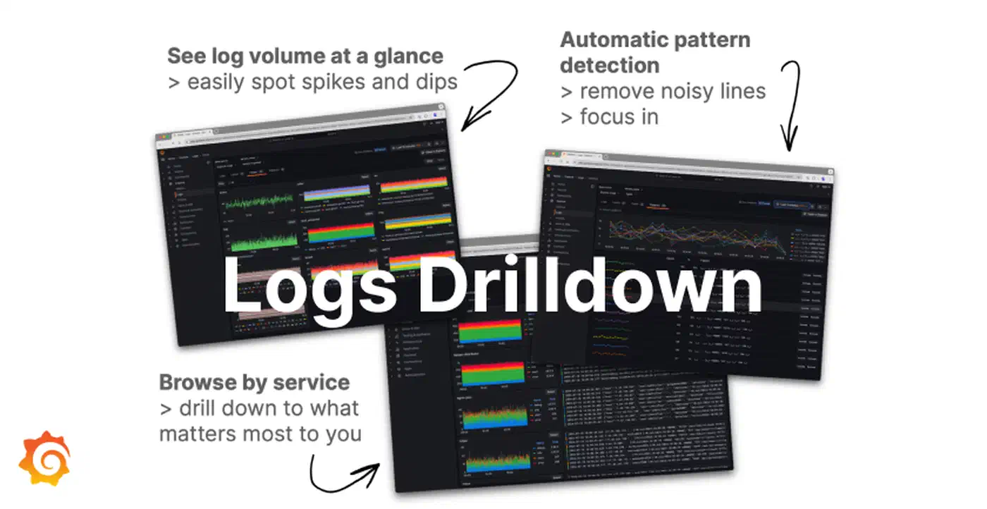

Journald Integration

For systems that use systemd, the python-systemd library provides direct access to systemd.journal.Reader. This is more efficient than spawning journalctl as a subprocess because you avoid the serialization overhead and get native Python objects:

from systemd import journal

reader = journal.Reader()
reader.add_match(_SYSTEMD_UNIT="myapp.service")
reader.seek_realtime(start_time)

entries = []
for entry in reader:
    if entry["__REALTIME_TIMESTAMP"] > end_time:
        break
    entries.append({
        "timestamp": entry["__REALTIME_TIMESTAMP"].isoformat(),
        "message": entry.get("MESSAGE", ""),
        "priority": entry.get("PRIORITY", 6),
        "unit": entry.get("_SYSTEMD_UNIT", "unknown"),
    })

Chunked Analysis for Large Log Volumes

When the preprocessed log set exceeds the context window, split it into chunks of roughly 1,500 lines with 100-line overlap between consecutive chunks. Analyze each chunk independently, then run a final meta-analysis pass that takes the summaries from all chunks and synthesizes them into a unified report. The overlap ensures that events spanning a chunk boundary are not missed.

def chunked_analyze(logs, chunk_size=1500, overlap=100):
    chunks = []
    for i in range(0, len(logs), chunk_size - overlap):
        chunks.append(logs[i : i + chunk_size])

    chunk_results = []
    for i, chunk in enumerate(chunks):
        result = analyze_with_ollama(chunk, model, anomaly_prompt)
        chunk_results.append(result)

    # Meta-analysis pass
    meta_prompt = f"Synthesize these {len(chunk_results)} analysis results..."
    final = analyze_with_ollama(chunk_results, model, meta_prompt)
    return final

Caching With SQLite

Repeated queries against the same log window during a post-mortem are common - you refine the prompt, add context, try different analysis angles. Store results in a local SQLite database keyed by a tuple of time range, services, analysis type, and a hash of the log content. Subsequent identical queries return instantly without re-running inference.

Incident Management Integration

Add a --post-incident flag that formats the LLM analysis into a structured incident report and posts it as a comment on the active incident via the PagerDuty API or Opsgenie API . This turns the analysis tool into part of your incident response workflow rather than a separate step someone has to remember to run. The same pattern - automating workflows with local LLMs via a CI pipeline - translates directly to other repetitive analysis tasks beyond log investigation.

Real-World Examples and Limitations

The following examples come from sanitized production incidents and show both what the approach gets right and where it breaks down.

Connection Pool Exhaustion

In this scenario, a FastAPI application started returning 502 errors after a deployment at 14:30. The logs contained no obvious error messages from the application itself - just nginx reporting upstream connection failures. When the interleaved logs from nginx, the FastAPI app, and PostgreSQL were fed to Llama 3.3 70B, it identified that PostgreSQL’s max_connections limit of 100 was reached because the new deployment introduced an async endpoint that opened database connections without properly returning them to the pool (missing async with around the connection context manager). The model traced the timeline from the deployment event through the gradual connection count increase to the eventual pool exhaustion and 502 cascade.

Disk Space Alert

A simpler case: the model correlated a No space left on device error in application logs with rapidly growing /var/log/nginx/access.log entries. It noticed that the access log file size was referenced in a monitoring log entry as 47GB and correctly identified that logrotate was not configured for this log path. It recommended both immediate cleanup with truncate -s 0 and adding a logrotate configuration to prevent recurrence.

Subtle Performance Degradation

The third example is subtler. A 30% increase in p99 response time appeared with zero error-level log entries. The model noticed that DNS resolution log entries (from a verbose application logger) showed resolution times jumping from 2ms to 200ms starting at the exact timestamp when a configuration management tool pushed a new resolv.conf. The misconfigured DNS server was the root cause - something that would have taken hours of manual investigation to correlate.

Where It Falls Apart

LLMs sometimes hallucinate causal relationships between events that happen to be close in time but are actually unrelated. A deployment and an unrelated DNS blip occurring within the same minute might get linked in the model’s analysis when they have nothing to do with each other. Always verify the model’s hypotheses against the actual log lines it cites.

Numerical precision is another weak point. Models struggle with accurate percentile calculations and rate computations. If you need to know that the p99 latency was exactly 342ms, use awk or pandas . Use the LLM for pattern recognition and hypothesis generation, not for math.

Context window constraints remain the fundamental limitation. Even with 128K tokens, a busy production system can generate millions of log lines in a 15-minute window. The preprocessing and sampling steps described earlier are not just nice-to-haves - they are mandatory. And they can introduce blind spots if the sampling strategy happens to filter out the one log line that explains everything.

With those caveats understood, LLM-powered log analysis still fills a practical gap between “I know exactly what to grep for” and paying Datadog $5,000 a month for anomaly detection. For teams already running Ollama for other tasks, adding log analysis is a low-effort extension. You will appreciate it the first time you are troubleshooting a 3 AM incident and want a second opinion on what the logs are saying.