AI-Powered Log Analysis: Find Anomalies in Server Logs with Local LLMs

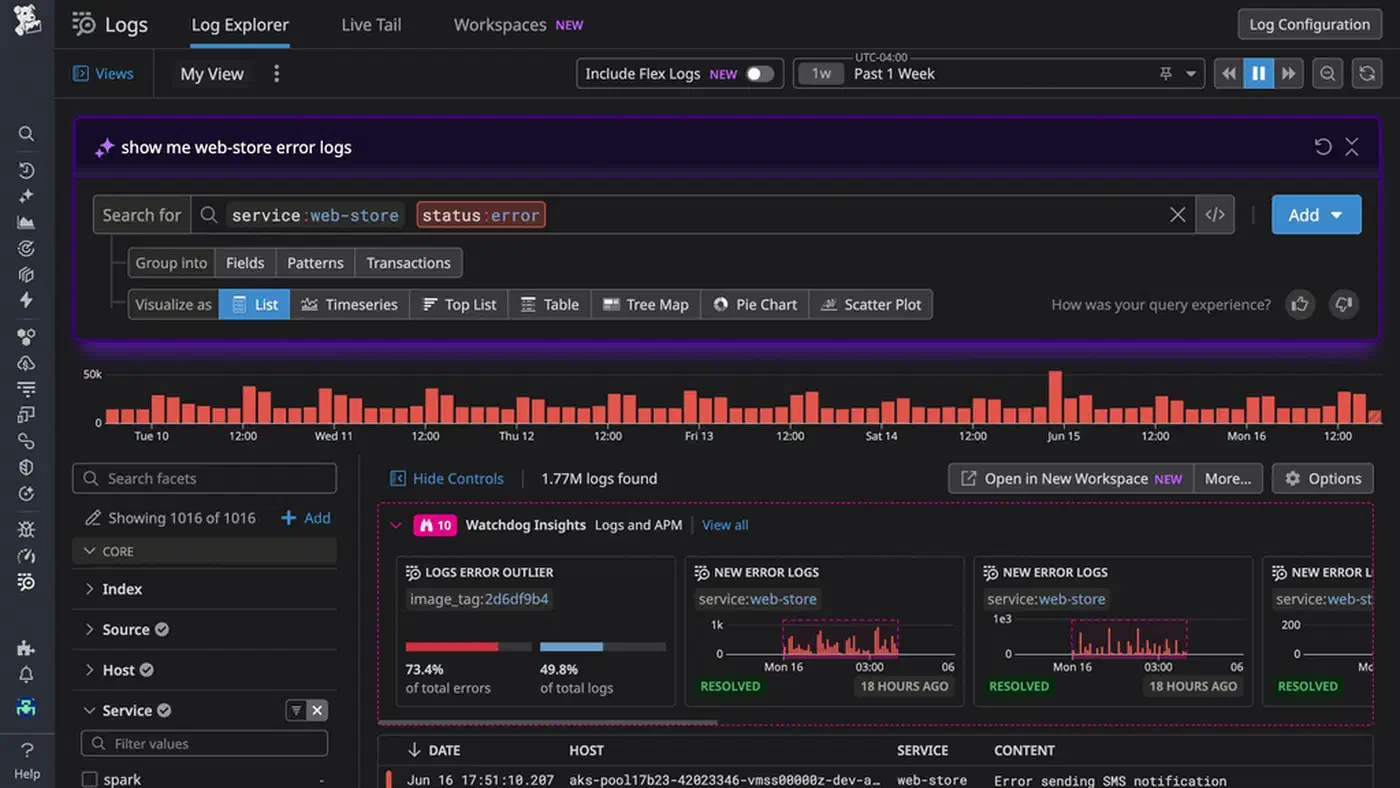
A local LLM like Llama 3.3 70B or Qwen 2.5 32B running through Ollama can read your structured server logs faster than grep or awk. Pipe parsed log data through a prompt that asks the model to flag odd patterns, link error cascades, and guess at root causes. You get a useful incident summary in seconds. This fills the gap between plain text search and pricey tools like Datadog or Splunk . Best of all, no log data leaves your network.

Why LLMs Beat Grep for Log Analysis

Tools like grep, awk, and jq need you to know the error string or pattern you want. That works when you know what broke. It falls apart when the bug is new, or when the symptom is a subtle shift in behavior rather than a clear error message.

LLMs spot anomalies by reading context. A 10x spike in 200 OK responses with 3-second latencies is invisible to grep. There is no error string to match. But a model asked to find “unusual patterns” in structured logs will flag it right away. It knows that 3-second response times on an endpoint that normally returns in 50ms is wrong, even though the HTTP status code looks fine.

LLMs also link events across services well. Feed mixed logs from nginx, a Python backend, and PostgreSQL into one prompt. The model can spot that a connection pool ran out at 14:32:05, and that this caused the 502 errors two seconds later at 14:32:07. Doing this by hand with grep means jumping between three log files and rebuilding the timeline in your head. The LLM does it in one pass.

The sweet spot for LLM log work is post-incident review and ad-hoc digging. It is not a swap for real-time alerts. A 70B model takes 10 to 30 seconds to read 5,000 log lines. That is fine for a post-mortem, but way too slow for a streaming pipeline that needs sub-second response. Use Loki and Grafana Alloy to collect and store logs, Grafana for dashboards and alerts, then point an LLM at one time window when something looks off. The LLM is the analyst, not the monitor.

Running models on your own box has a serious privacy upside. Production logs hold IP addresses, user IDs, session tokens, and sometimes API keys that slipped into a debug line. Sending those to a cloud LLM (even with a Data Processing Agreement) is a risk you do not need to take. A local Ollama instance keeps every byte on your own hardware.

The cost math is simple too. Datadog Log Management charges $0.10 per GB ingested, plus $1.70 per million log events for analysis. A box running Ollama with a decent GPU costs a fixed amount per month: about $200 based on your hardware. That price holds no matter how many logs you process. Once you cross a few GB of logs per day, the local setup pays for itself fast.

Preparing Logs for LLM Consumption

Raw log files are noisy, formatted in odd ways, and burn through context tokens. Preprocessing is not a nice-to-have. It is the line between useful analysis and the model drowning in health check entries.

Parsing Into Structured JSON

The first step is turning raw logs into JSON with fixed fields. Vector (open source, first built by Datadog) and Fluent Bit both do this well. The goal is to map syslog, nginx access logs, and app logs into JSON lines with a shared schema: timestamp, level, service, message, and metadata.

A Vector configuration for parsing nginx access logs looks something like this:

[sources.nginx_logs]
type = "file"
include = ["/var/log/nginx/access.log"]

[transforms.parse_nginx]
type = "remap"
inputs = ["nginx_logs"]
source = '''
. = parse_nginx_log!(.message, "combined")
.service = "nginx"
.level = if .status >= 500 { "ERROR" } else if .status >= 400 { "WARN" } else { "INFO" }
'''

Filtering Out Noise

Before anything hits the LLM, filter hard. Use jq or Vector transforms to drop DEBUG messages, health check pings (GET /healthz), and static assets (CSS, JS, images). They add noise with no diagnostic value. In a typical web app, dropping health checks and static assets alone cuts log volume by 40 to 60%.

Time-Window Extraction

When you dig into an incident, pull a tight window rather than hours of logs. Five minutes before to ten minutes after the first alert is plenty for the first pass. With journald:

journalctl --since "2026-03-28 14:30:00" \
           --until "2026-03-28 14:45:00" \
           -o json

Token Budget Planning

Structured JSON logs run 50 to 100 tokens per line. A 128K context window (Llama 3.3) fits about 1,500 to 2,500 log lines plus the system prompt and the model’s reply. That covers most focused digs. For longer windows you will need chunked analysis (see the pipeline section below).

Deduplication

This is one of the biggest wins for token use. Fold repeated identical log lines into one entry with a count field:

{
  "message": "Connection refused to db-primary:5432",
  "count": 847,
  "first_seen": "14:32:05",
  "last_seen": "14:33:12"
}

Rather than burn 847 lines of tokens on the same message, you use one line. The model still gets that this error fired 847 times in about a minute. That count tells you more than seeing each one in full.

Sampling for Large Volumes

If the window holds 50,000+ lines even after filtering, you need a sampling plan. Take the first and last 500 lines in full (to catch the start and end of the incident). Then sample every Nth line from the middle, weighted toward ERROR and WARN. This keeps the timeline intact while fitting the context budget.

Prompting Strategies for Log Analysis

LLM log analysis lives or dies by the prompt. A vague “analyze these logs” prompt gives vague results. A clear, structured prompt gives output you can act on during an incident.

Anomaly Detection

This prompt template works well for initial triage:

You are a senior SRE analyzing server logs. Below are structured log
entries from [services] between [time range]. Identify any anomalous
patterns, unexpected error rates, latency spikes, or unusual sequences.

For each anomaly, state:
1. What is abnormal
2. The affected time range
3. Which services are involved
4. Your confidence level (high/medium/low)

Root-Cause Analysis

For deeper investigation after you have identified the problem window:

Given the following log entries showing a service degradation starting
at [time], trace the chain of events backward from the user-visible
symptom to the likely root cause.

Present your analysis as a numbered timeline with causal relationships
marked.

Structured Output

Free-form text replies are hard to wire into scripts. Use JSON mode or a library like Instructor so the model returns parseable results. If you are new to structured LLM output, our guide on JSON schemas and the Instructor library covers the full setup, with Pydantic models and auto-retry on validation failure. Define a schema like this:

{
  "anomalies": [
    {
      "description": "string",
      "severity": "high|medium|low",
      "time_range": "string",
      "affected_services": ["string"],
      "evidence_lines": ["string"],
      "hypothesis": "string"
    }
  ]
}

Now you can pipe the LLM output straight into a script that creates PagerDuty notes or Grafana dashboard markers.

Few-Shot Examples

Adding 2 or 3 examples of annotated log snippets with their expected analysis to the system prompt lifts accuracy a lot. The model copies the style and output format from your examples. This is great for teaching the model about your own stack. If your load balancer logs use an odd format or your app has custom error codes, a few examples go a long way.

Chain-of-Thought for Complex Investigations

For multi-service correlation, walk the model through a clear process:

Think step by step. First, identify all error-level events. Then, look
for temporal correlations between services. Then, check for cascading
failures where an error in one service causes errors in dependent services.
Finally, identify the earliest event in the chain as the likely root cause.

Model Selection

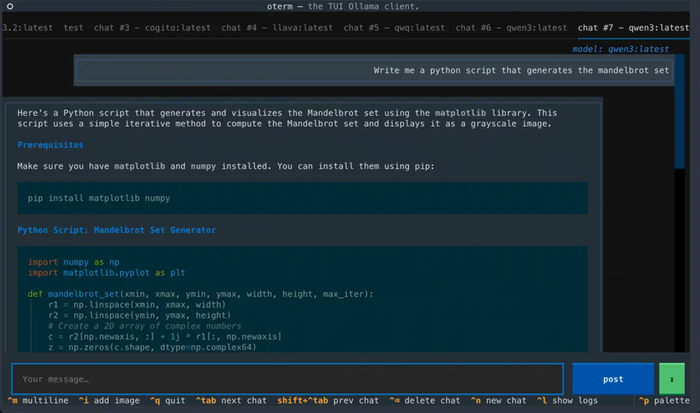
For log analysis, Qwen 2.5 32B Instruct (Q5_K_M, about 24GB of RAM) gives the best accuracy per gigabyte for structured tasks. Llama 3.3 70B (Q4_K_M, about 40GB RAM) is better for thick multi-service work. It holds more context and reasons over longer chains. Skip models below 14B for this job. They miss subtle patterns and give shallow results. If you have a 128GB unified-memory box and want a stronger reasoning model for incident-response agents, the MiniMax M2.7 self-evolving model runs offline and is tuned for exactly this kind of long-context agent work. If your box only has a small card, the offload approach for running Gemma 4 26B MoE on 8GB VRAM gets a capable model onto modest hardware. For a side-by-side of model sizes and hardware needs when running models locally with Ollama , with benchmarks across GPU tiers, that guide shows what to expect before you pick a size.

Building the Analysis Pipeline

Good prompts are one thing. Making the whole flow fast and repeatable enough to use during a real incident is another. Here is how to wire it all into a working pipeline.

CLI Tool Architecture

The core tool is a Python script. It takes a time range, a service filter, and an analysis type (anomaly detection, root-cause, or summary). It pulls logs from journald or Loki, runs them through preprocessing, and streams the LLM reply to your terminal.

import argparse
import json
import httpx
from datetime import datetime

def fetch_from_loki(endpoint, query, start, end):
    """Fetch logs from Loki HTTP API."""
    resp = httpx.get(
        f"{endpoint}/loki/api/v1/query_range",
        params={
            "query": query,
            "start": start.isoformat() + "Z",
            "end": end.isoformat() + "Z",
            "limit": 5000,
        },
    )
    resp.raise_for_status()
    return parse_loki_response(resp.json())

def analyze_with_ollama(logs, model, prompt_template):
    """Stream analysis from local Ollama instance."""
    prompt = prompt_template.format(logs=json.dumps(logs, indent=2))
    with httpx.stream(
        "POST",
        "http://localhost:11434/api/generate",
        json={"model": model, "prompt": prompt, "stream": True},
        timeout=120,
    ) as resp:
        for line in resp.iter_lines():
            chunk = json.loads(line)
            print(chunk.get("response", ""), end="", flush=True)

Loki Integration

The Loki HTTP API takes LogQL queries via GET /loki/api/v1/query_range. You can filter by label (service name, environment) and by content (grep-like filters inside LogQL). The reply comes back as JSON. Flatten it into the structured format your prompts expect.

A typical LogQL query for incident investigation:

{service="api-gateway"} |= "error" | json | level="ERROR"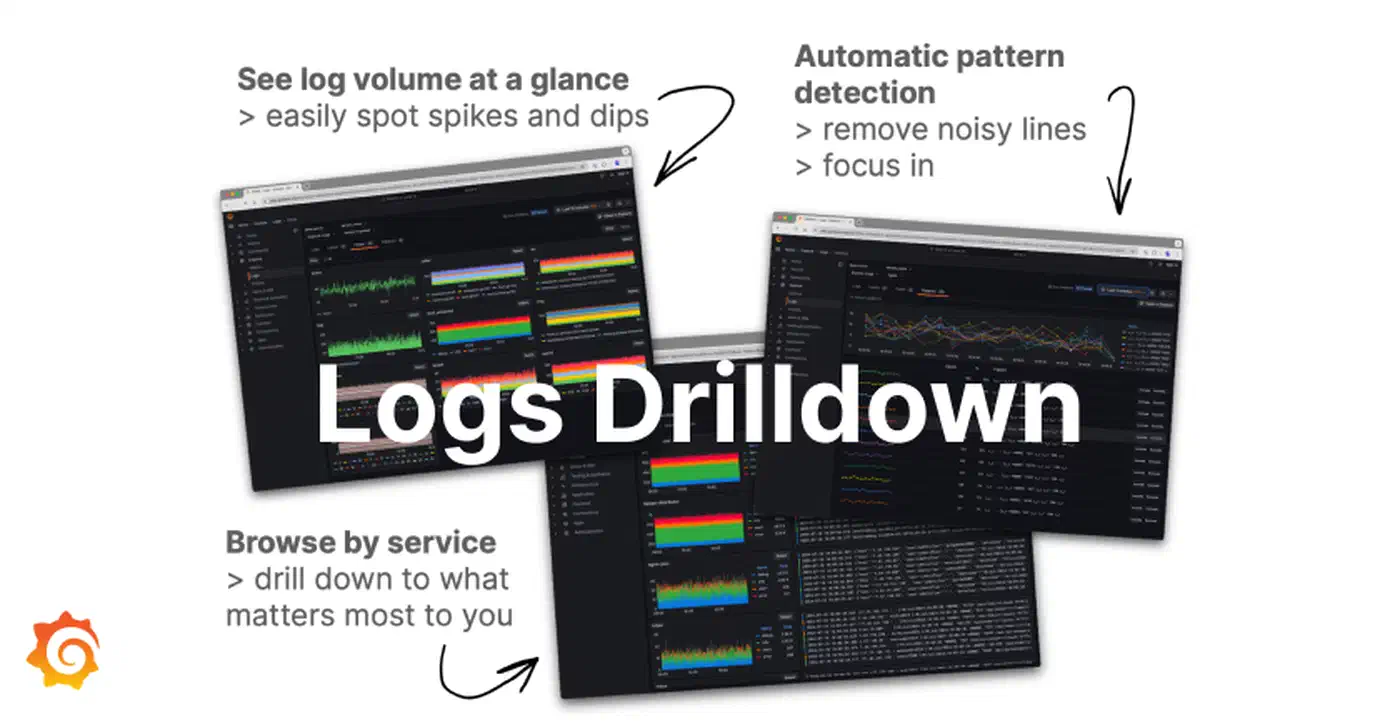

Journald Integration

On systemd boxes, the python-systemd library gives you direct access to systemd.journal.Reader. This beats spawning journalctl as a subprocess. You skip the serialization overhead and you get native Python objects:

from systemd import journal

reader = journal.Reader()
reader.add_match(_SYSTEMD_UNIT="myapp.service")
reader.seek_realtime(start_time)

entries = []
for entry in reader:
    if entry["__REALTIME_TIMESTAMP"] > end_time:
        break
    entries.append({
        "timestamp": entry["__REALTIME_TIMESTAMP"].isoformat(),
        "message": entry.get("MESSAGE", ""),
        "priority": entry.get("PRIORITY", 6),
        "unit": entry.get("_SYSTEMD_UNIT", "unknown"),
    })

Chunked Analysis for Large Log Volumes

When the cleaned log set is bigger than the context window, split it into chunks of about 1,500 lines with 100-line overlap between chunks. Analyze each chunk on its own. Then run a final meta pass that pulls the chunk summaries into one report. The overlap stops you missing events that straddle a chunk boundary.

def chunked_analyze(logs, chunk_size=1500, overlap=100):
    chunks = []
    for i in range(0, len(logs), chunk_size - overlap):
        chunks.append(logs[i : i + chunk_size])

    chunk_results = []
    for i, chunk in enumerate(chunks):
        result = analyze_with_ollama(chunk, model, anomaly_prompt)
        chunk_results.append(result)

    # Meta-analysis pass
    meta_prompt = f"Synthesize these {len(chunk_results)} analysis results..."
    final = analyze_with_ollama(chunk_results, model, meta_prompt)
    return final

Caching With SQLite

Repeated queries on the same log window are common in a post-mortem. You tweak the prompt, add context, try new angles. Store results in a local SQLite database keyed by a tuple: time range, services, analysis type, and a hash of the log content. Later identical queries return at once, with no fresh inference run.

Incident Management Integration

Add a --post-incident flag. It formats the LLM analysis into a clean incident report and posts it as a comment on the active incident via the PagerDuty API or Opsgenie API . Now the tool sits inside your incident response, not as an extra step someone has to remember. The same pattern, automating workflows with local LLMs via a CI pipeline , maps directly to other rote analysis tasks beyond logs.

Real-World Examples and Limitations

These examples come from sanitized production incidents. They show what the method gets right, and where it breaks down.

Connection Pool Exhaustion

In this case, a FastAPI app started returning 502 errors after a deploy at 14:30. The app logs held no clear error message. Just nginx reporting upstream connection failures. Mixed logs from nginx, the FastAPI app, and PostgreSQL went into Llama 3.3 70B. The model flagged that PostgreSQL hit its max_connections limit of 100. The new deploy added an async endpoint that opened database connections without returning them to the pool. The bug was a missing async with around the connection context manager. The model traced the timeline from deploy, through the slow climb in connection count, to the pool running dry and the 502 cascade.

Disk Space Alert

A simpler case. The model linked a No space left on device error in app logs with fast-growing /var/log/nginx/access.log entries. It saw that a monitoring log entry pegged the access log file size at 47GB. It correctly flagged that logrotate was not set up for this log path. It suggested both a quick cleanup with truncate -s 0 and adding a logrotate config to stop a repeat.

Subtle Performance Degradation

The third case is subtler. A 30% rise in p99 response time showed up with zero error-level entries. The model spotted that DNS resolution log entries (from a chatty app logger) showed times jumping from 2ms to 200ms. They jumped at the exact moment a config management tool pushed a new resolv.conf. The wrong DNS server was the root cause. By hand, that link would have taken hours to find.

Where It Falls Apart

LLMs sometimes hallucinate causal links between events that sit close in time but are not related. A deploy and a stray DNS blip in the same minute can get linked in the model’s reply, when they have nothing to do with each other. Always check the model’s claims against the log lines it cites.

Numeric precision is another weak spot. Models trip up on exact percentile math and rate counts. If you need to know that p99 latency was exactly 342ms, reach for awk or pandas . Use the LLM for spotting patterns and guessing causes, not for math.

Context window limits are the core constraint. Even with 128K tokens, a busy production system can spit out millions of log lines in a 15-minute window. The preprocessing and sampling steps above are not optional. They are required. They can also create blind spots, if the sampling plan happens to drop the one log line that explains it all.

With those caveats in mind, LLM log analysis still fills a real gap. The gap sits between “I know exactly what to grep for” and paying Datadog $5,000 a month for anomaly detection. For teams already running Ollama for other tasks, adding log analysis is a small extra step. You will be glad you have it the first time you are at a 3 AM incident and want a second opinion on what the logs say.