 Botmonster Tech
Postgres 18 can replace Redis, Kafka, and Elasticsearch


A single Postgres 18
instance with a few extensions can replace Redis, Kafka, MongoDB, Elasticsearch, Pinecone, Qdrant, InfluxDB, and most of your custom API tier. The core pieces are JSONB with GIN for schemaless data, SELECT FOR UPDATE SKIP LOCKED for queues, tsvector and pg_trgm for search, and pgvector 0.8 for vector queries. PostGIS
, partitioning with BRIN, concurrent materialized views, and PostgREST or pg_graphql with Row-Level Security cover the rest. You back up and monitor one database, not eight. Most teams cut 40-60% of running cost until they hit true distributed scale.
Why “just use Postgres” became the default stack
For most of the last decade, a greenfield web app spread its data across half a dozen services. Postgres held the rows, Redis ran cache and queues, RabbitMQ or Kafka carried events. Elasticsearch ran search, MongoDB held schemaless data, Pinecone held vectors, and InfluxDB held telemetry. A handwritten Node or Python tier glued it all together. Each piece solved a real problem. Together they shipped a dozen vendor invoices and a steady run of cross-system bugs that ate part of each sprint.
A few forces flipped that default. Postgres 16 shipped vector-friendly tweaks. Version 17 added incremental backups and better JSON path queries. Version 18 brought async I/O , skip-scan B-tree reads , virtual generated columns, and native UUIDv7. The extension list also grew: pgvector, PostGIS, TimescaleDB, pg_trgm, pg_cron, pg_partman, pg_graphql, PostgREST, pgaudit, and poolers like PgCat or Supavisor. Together they cover almost any workload a backend sees.
The biggest draw is ACID across features. Your queue, your vectors, and your rows all commit in one transaction. No polyglot stack can offer that. A failed job no longer leaves an orphan row, a duplicate Kafka message, or a stale embedding. Ops gets simpler too. You keep one backup and HA plan, one monitoring stack, and you hire for a single skillset instead of eight.
The case has real limits. Petabyte-scale columnar analytics, multi-region active-active writes, and Prometheus-level metric counts still want their own tools. The last section covers those edges.
Replace MongoDB with JSONB and GIN indexes
Document stores exist for flexible, nested, changing schemas. Postgres has had a first-class binary JSON type since 9.4. Today it beats MongoDB on most OLTP workloads and keeps full ACID rules. You can also join documents against plain tables in one query.
JSONB stores documents in a parsed binary format at insert time, so reads don’t re-parse it each time. The older text-based json type loses on exactly that. A GIN (Generalized Inverted Index) turns a JSONB column into a real document store. The index maps each key-value pair to the rows that hold it. Lookups on deeply nested fields land in under a millisecond. Two operator classes cover most cases. jsonb_ops is the default and has the widest set of operators. jsonb_path_ops builds a smaller index that runs containment (@>) queries faster, but only for that operator group.
A common pattern for mixed event payloads looks like this:
CREATE TABLE events (
  id         bigserial PRIMARY KEY,
  created_at timestamptz NOT NULL DEFAULT now(),
  payload    jsonb NOT NULL
);

CREATE INDEX events_payload_gin ON events USING gin (payload jsonb_path_ops);

SELECT id, payload
FROM events
WHERE payload @> '{"user_id": 42, "type": "signup"}'
ORDER BY created_at DESC
LIMIT 50;
A well-indexed JSONB table answers that containment query in single-digit milliseconds across tens of millions of rows. For the two or three fields you query most, a generated column plus a B-tree index often beats a GIN index. It also takes less disk:
ALTER TABLE events
  ADD COLUMN user_id bigint
  GENERATED ALWAYS AS ((payload->>'user_id')::bigint) STORED;

CREATE INDEX ON events (user_id, created_at DESC);
Generated columns and indexes like these are schema changes. Wrap each ALTER TABLE in a version-controlled migration script
instead of running it by hand in production. A GIN index on JSONB covers structure rather than language, so long text fields buried inside docs still want tsvector, covered below.
Replace Redis and RabbitMQ with SKIP LOCKED
Background jobs are the biggest reason teams reach for Redis or RabbitMQ. Postgres ships a locking clause that turns a plain table into a fast queue. It also avoids the classic “two workers grab the same row” bug. That failure mode sank naive setups years ago.
FOR UPDATE SKIP LOCKED works at the MVCC level. The first transaction grabs a row-level lock on the tuples it reads. Other workers running the same query skip the locked rows and pick up the next ones. Nothing blocks, and you write no extra glue code in the app.
SELECT id, payload
FROM jobs
WHERE status = 'pending'
  AND run_after <= now()
ORDER BY priority DESC, created_at
FOR UPDATE SKIP LOCKED
LIMIT 10;
A well-tuned Postgres cluster handles tens of thousands of jobs per second on one box. That ceiling sits above almost any app workload short of ad-serving or realtime bidding. Unlogged staging tables, eager autovacuum, and partial indexes on status = 'pending' push it higher.
Many mature libraries bake in the pattern. pgmq
covers raw SQL consumers. River
ships in Go, Oban
in Elixir, GoodJob
and Solid Queue
in Rails, graphile-worker
in Node, and procrastinate
in Python. For cron-style runs, pg_cron
lives in the database. It fires jobs on the same schedule every other feature already uses. LISTEN/NOTIFY wakes workers fast with no poll loop. That’s the 2026 take on pub/sub for most in-app cases
.
Redis and Kafka still win for sub-millisecond hot caches feeding millions of websocket fanouts. They also win for multi-day event logs with replayable consumer groups, and for cross-region streaming. Without those needs, a Postgres queue is almost always the right call.
Replace Elasticsearch with tsvector, pg_trgm, and ParadeDB
Elasticsearch is a great product that most apps don’t need. Between core Postgres full-text search and the newer BM25 extensions, a basic search bar has no business needing a second cluster.
Core Postgres ships tsvector and tsquery types. They handle language-aware tokens, stop-word removal, stemming (running becomes run), and ranking via ts_rank and ts_rank_cd. A GIN index over a tsvector column answers queries in under a millisecond across millions of docs. The pg_trgm
extension adds trigram match for fuzzy search that forgives typos. postgress still finds postgresql, and partial matches work. A GiST or GIN index keeps it fast. Stored generated tsvector columns keep things in sync on their own:
ALTER TABLE articles
  ADD COLUMN search tsvector
  GENERATED ALWAYS AS (
    setweight(to_tsvector('english', coalesce(title, '')),  'A') ||
    setweight(to_tsvector('english', coalesce(body,  '')),  'B')
  ) STORED;

CREATE INDEX articles_search_gin ON articles USING gin (search);

SELECT id, title, ts_rank_cd(search, q) AS rank
FROM articles, plainto_tsquery('english', 'postgres vector search') AS q
WHERE search @@ q
ORDER BY rank DESC
LIMIT 20;
For ranking-heavy apps where ts_rank feels crude, two recent extensions close the gap. ParadeDB’s pg_search
brings Elasticsearch-grade BM25 scoring into the database. It wraps the Tantivy search library
as a Postgres index type. Tiger Data’s pg_textsearch
takes a different path. It writes a full BM25 engine in C, on top of Postgres storage. Tiger Data reports
2.4x to 6.5x faster queries than ParadeDB at 138 million documents. Either way, BM25 now lives inside the same transaction as the rest of your data.
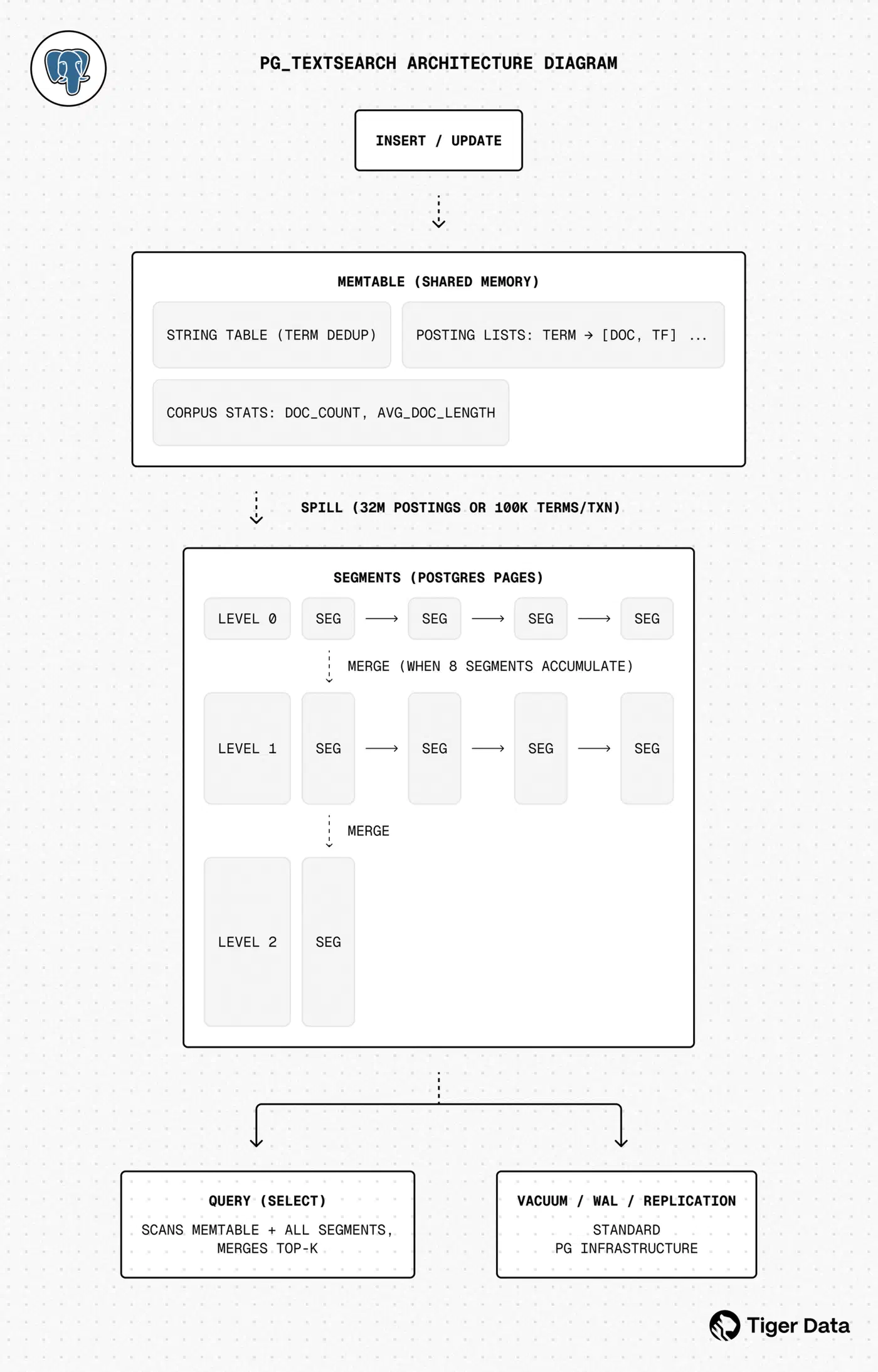
Here is how the feature matrix looks in practice:
| Workload | Postgres feature / extension | Realistic ceiling on one node | When to escape |
|---|---|---|---|
| Exact and prefix search | tsvector + GIN | Tens of millions of docs | Petabyte log analytics |
| Fuzzy / typo-tolerant | pg_trgm + GiST | Millions of names / strings | Dedicated fuzzy engines |
| BM25 relevance ranking | pg_search (ParadeDB) / pg_textsearch | Hundreds of millions of docs | Globally distributed tenants |
| Faceted / aggregation-heavy | Postgres + materialized views | Hundreds of millions of rows | Complex geo+text faceting at scale |
Replace Pinecone with pgvector 0.8
Keeping vectors in a second database creates the “hybrid search problem”. Each semantic query has to cross-check row data over the network. That check often lands in app code, a reliable source of bugs. pgvector fixes that. Vectors become just another column, joinable in one ACID query.
pgvector 0.8.0 shipped three big changes. Iterative index scans
fix the old footgun where a tight WHERE filter would kill recall. The old scan dropped too many HNSW candidates before the result set was full. The new halfvec type stores 2-byte floats, which halves memory and lets indexes go up to 16,000 dims with tiny recall loss. A sparsevec type covers keyword-style embeddings.
HNSW is a Hierarchical Navigable Small World graph. It stacks layers and acts like a skip list in many dimensions. You get sub-linear approximate nearest neighbor search. Three knobs tune it: m, ef_construction, and ef_search.
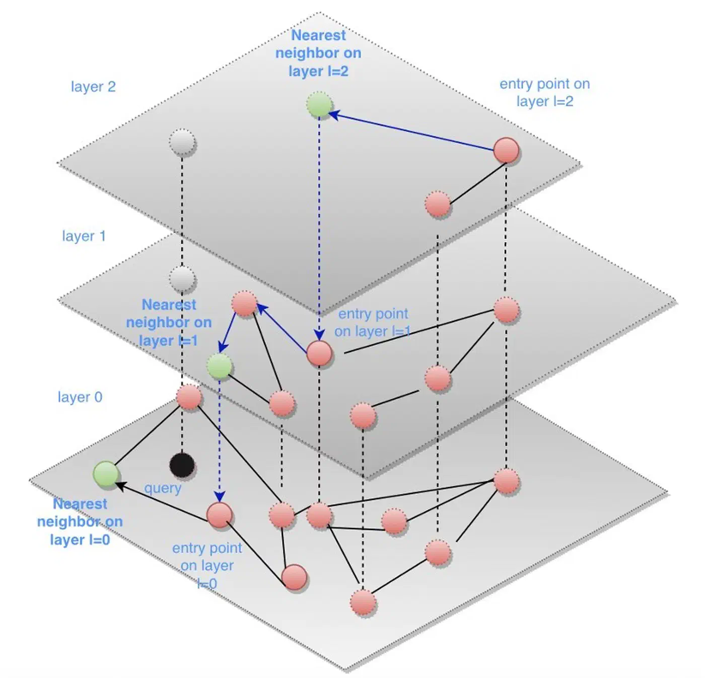
Hybrid queries are where this pays off. One SQL statement can rank by vector distance and filter by tenant_id, created_at, or a PostGIS polygon, in one round trip with ACID intact:
SELECT id, title, embedding <=> $1 AS distance
FROM documents
WHERE tenant_id = $2
  AND created_at > now() - interval '90 days'
ORDER BY embedding <=> $1
LIMIT 10;
With SET hnsw.iterative_scan = 'relaxed_order' and a sane hnsw.max_scan_tuples, that query stays fast even when the filter is very selective. Filtered queries used to be the worst case for pgvector, and iterative scans make them run up to 9x faster.
For vector sets that outgrow RAM, pgvectorscale adds StreamingDiskANN. It’s a disk-based index built for larger-than-memory loads. Binary quantization shrinks storage by about 32x with little recall loss on well-trained embedding models. Embeddings sit next to the rows they describe. The whole class of “dual-write sync job drifted overnight” outages goes away.
Replace dedicated GIS and BI with PostGIS and materialized views
PostGIS has been the gold standard for map data in SQL databases since before most GIS products shipped. Pair it with materialized views for reports. Postgres then handles the map and report work that teams often overpay vendors to solve.
The GiST (Generalized Search Tree) index in PostGIS does a cheap bounding-box pre-filter on complex shapes. Only then does it run exact distance math. That’s why “coffee shops in this polygon” queries finish in milliseconds across millions of features. The geometry type uses planar math, fast and often fine for city-scale work. The geography type does spheroid math, so pick it when you need accuracy across a continent. pgRouting
handles shortest-path and network routing. h3-pg
brings Uber’s hexagonal spatial index into Postgres.
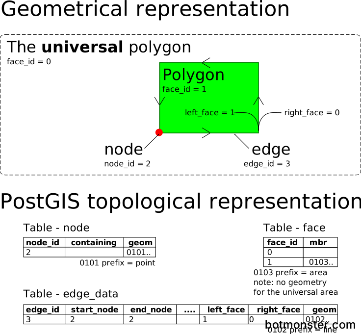
Materialized views drop the need for a second BI warehouse on small-to-medium datasets. Run the heavy math once, store the result on disk, and serve dashboard reads from a ready-made table:
CREATE MATERIALIZED VIEW daily_signups AS
SELECT date_trunc('day', created_at) AS day,
       country,
       count(*) AS signups
FROM users
GROUP BY 1, 2;

CREATE UNIQUE INDEX ON daily_signups (day, country);

REFRESH MATERIALIZED VIEW CONCURRENTLY daily_signups;
The CONCURRENTLY flag swaps rows in without blocking readers, though it needs a unique index. Trigger the refresh from pg_cron on a schedule, or from app code when upstream writes land. Past a billion rows, columnar OLAP engines like DuckDB, ClickHouse, or Snowflake still win. Same goes when sub-second ad-hoc reports on any field become the headline need. Postgres 18’s better parallel query planner and TimescaleDB’s configurable columnstore
have shrunk that gap a lot.
Replace time-series databases with partitioning and BRIN
Billions of telemetry events feel like they need a purpose-built time-series database. Most teams don’t need one. Native range partitioning plus a BRIN index on the timestamp column does the job, at a fraction of the cost to run.
Range partitioning routes inserts to the right child partition on its own. Queries also prune unused partitions at planning time. pg_partman handles the upkeep. It creates next month’s partition, drops old ones past the cutoff, and compresses closed chunks.
BRIN (Block Range Index) stores only the min and max values for each block range on disk. On a billion-row timestamp column with time-ordered inserts, a BRIN index is orders of magnitude smaller than the matching B-tree. It stays nearly as selective for range queries. With partitioning, BRIN, and unlogged staging tables in front of the main table, a well-tuned Postgres node ingests hundreds of thousands of events per second.
CREATE TABLE metrics (
  ts     timestamptz NOT NULL,
  host   text NOT NULL,
  metric text NOT NULL,
  value  double precision
) PARTITION BY RANGE (ts);

CREATE INDEX ON metrics USING brin (ts) WITH (pages_per_range = 32);
When plain partitioning is not enough, TimescaleDB steps in. It adds hypertables, continuous aggregates, and columnar compression up to 95%, all still inside Postgres. Prometheus, VictoriaMetrics, or Mimir still win when metric labels blow up in count. They also win when you need purpose-built downsampling rules, or the exact shape of PromQL math at scale.
Replace your API tier with PostgREST, pg_graphql, and RLS
The middle tier can go too. A typical CRUD app carries thousands of lines of Node or Python boilerplate. Its only job is to shuffle rows between Postgres and JSON. Some tools read your schema and generate a correct, safe API, which drops that layer for good. Pair them with Row-Level Security and you’re done.
PostgREST reads your schema and serves a fully documented REST API. You get filters, pagination, ordering, related-resource embedding, bulk inserts, and RPC calls. pg_graphql applies the same idea to GraphQL. It lives as a Postgres extension, so the API itself is part of the database. Both use the same permission system as the rest of Postgres. Access rules stay in one place.
Row-Level Security policies are per-table rules. Postgres checks each one against the caller’s ID, often passed in as JWT claims:
ALTER TABLE orders ENABLE ROW LEVEL SECURITY;

CREATE POLICY orders_owner
  ON orders
  FOR ALL
  USING (
    user_id = (current_setting('request.jwt.claims', true)::jsonb ->> 'user_id')::bigint
  );
With that one policy, a user can read and edit only their own orders. The rule fires no matter which client, script, or SQL console connects, though the clients themselves shift under you: the popular Chat2DB dropped its open license at version 5.3.0. Supabase , Nhost, and the wider PostgREST-based stacks prove this pattern holds up well beyond prototype scale. Where it breaks down is thick domain logic. Heavy business rules and multi-step flows still belong in app code, or in Postgres functions you call via RPC. So does anything that would be awkward as a plain SQL function.
The limits: when not to just use Postgres
“Just use Postgres” is a rule of thumb, and it has real edges. Knowing where those edges sit saves you from costly mistakes at scale.
Vertical scaling carries Postgres further than most people think. A 96-core box with fast NVMe handles huge throughput. Set shared_buffers near 25% of RAM, give effective_cache_size a big value, tune work_mem per workload, and put a pooler in front (PgBouncer, PgCat, or Supavisor). Horizontal sharding via Citus
or logical partitioning works, but it’s heavier to run than the marketing hints. That’s the first real cliff you hit.
Other places the pattern breaks:
- Hot-path caching under a millisecond for millions of live websocket clients: Redis and Dragonfly still own this ground.
- Durable event streaming with days of backlog and replayable consumer groups at scale: that is Kafka or Redpanda turf.
- Metrics with a huge number of label values: Prometheus paired with VictoriaMetrics or Mimir.
- Petabyte columnar analytics with sub-second ad-hoc queries: ClickHouse, DuckDB, or Snowflake.
- Multi-region active-active writes that stay fast everywhere: CockroachDB, Spanner, or YugabyteDB.
Start with Postgres. Add a specialized tool only when real numbers show one well-tuned box can’t serve the workload. When that day comes, the move costs less than the years of polyglot overhead you skipped. Managed options like Neon , Supabase, Tiger Cloud , Crunchy Bridge, AWS Aurora Postgres, and Google AlloyDB take on the ops work while you wait.
The stack that used to need six products now fits into one. A decade of extension work and core upgrades met a market that got tired of gluing things together.